As an entry point to learning python and getting into Machine Learning, I decided to code from scratch the Hello World! of the field, a single neuron perceptron.
What is a perceptron?
A perceptron is the basic building block of a neural network, it can be compared to a neuron, And its conception is what detonated the vast field of Artificial Intelligence nowadays.
Back in the late 1950’s, a young Frank Rosenblatt devised a very simple algorithm as a foundation to construct a machine that could learn to perform different tasks.
In its essence, a perceptron is nothing more than a collection of values and rules for passing information through them, but in its simplicity lies its power.
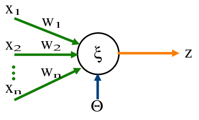
Imagine you have a ‘neuron’ and to ‘activate’ it, you pass through several input signals, each signal connects to the neuron through a synapse, once the signal is aggregated in the perceptron, it is then passed on to one or as many outputs as defined. A perceptron is but a neuron and its collection of synapses to get a signal into it and to modify a signal to pass on.
In more mathematical terms, a perceptron is an array of values (let’s call them weights), and the rules to apply such values to an input signal.
For instance a perceptron could get 3 different inputs as in the image, lets pretend that the inputs it receives as signal are: $x_1 = 1, \; x_2 = 2\; and \; x_3 = 3$, if it’s weights are $w_1 = 0.5,\; w_2 = 1\; and \; w_3 = -1$ respectively, then what the perceptron will do when the signal is received is to multiply each input value by its corresponding weight, then add them up.
\(
\begin{align}
\begin{split}
\left(x_1 * w_1\right) + \left(x_2 * w_2\right) + \left(x_3 * w_3\right)
\end{split}
\end{align}
\)
\(
\begin{align}
\begin{split}
\left(0.5 * 1\right) + \left(1 * 2\right) + \left(-1 * 3\right) = 0.5 + 2 - 3 = -0.5
\end{split}
\end{align}
\)
Typically when this value is obtained, we need to apply an “activation” function to smooth the output, but let’s say that our activation function is linear, meaning that we keep the value as it is, then that’s it, that is the output of the perceptron, -0.5.
In a practical application, the output means something, perhaps we want our perceptron to classify a set of data and if the perceptron outputs a negative number, then we know the data is of type A, and if it is a positive number then it is of type B.
Once we understand this, the magic starts to happen through a process called backpropagation, where we “educate” our tiny one neuron brain to have it learn how to do its job.
The magic starts to happen through a process called backpropagation, where we "educate" our tiny one neuron brain to have it learn how to do its job.
For this we need a set of data that it is already classified, we call this a training set. This data has inputs and their corresponding correct output. So we can tell the little brain when it misses in its prediction, and by doing so, we also adjust the weights a bit in the direction where we know the perceptron committed the mistake hoping that after many iterations like this the weights will be so that most of the predictions will be correct.
After the model trains successfully we can have it classify data it has never seen before, and we have a fairly high confidence that it will do so correctly.
The math behind this magical property of the perceptron is called gradient descent, and is just a bit of differential calculus that helps us convert the error the brain is having into tiny nudges of value of the weights towards their optimum. This video series by 3 blue 1 brown explains it wonderfuly.
My program creates a single neuron neural network tuned to guess if a point is above or below a randomly generated line and generates a visualization based on graphs to see how the neural network is learning through time.
The neuron has 3 inputs and weights to calculate its output:
input 1 is the X coordinate of the point,
Input 2 is the y coordinate of the point,
Input 3 is the bias and it is always 1

Input 3 or the bias is required for lines that do not cross the origin (0,0)
The Perceptron starts with weights all set to zero and learns by using 1,000 random points per each iteration.
The output of the perceptron is calculated with the following activation function:
if x * weight_x + y weight_y + weight_bias is positive then 1 else 0
The error for each point is calculated as the expected outcome of the perceptron minus the real outcome therefore there are only 3 possible error values:
| Expected |
Calculated |
Error |
| 1 |
-1 |
1 |
| 1 |
1 |
0 |
| -1 |
-1 |
0 |
| -1 |
1 |
-1 |
With every point that is learned if the error is not 0 the weights are adjusted according to:
New_weight = Old_weight + error * input * learning_rate
for example: New_weight_x = Old_weight_x + error * x * learning rate
A very useful parameter in all of neural networks is teh learning rate, which is basically a measure on how tiny our nudge to the weights is going to be.
In this particular case, I coded the learning_rate to decrease with every iteration as follows:
learning_rate = 0.01 / (iteration + 1)
this is important to ensure that once the weights are nearing the optimal values the adjustment in each iteration is subsequently more subtle.
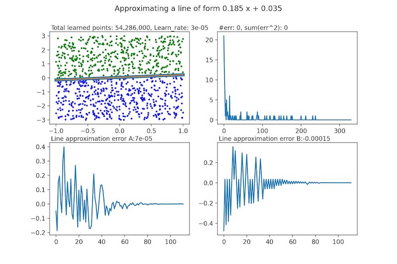
In the end, the perceptron always converges into a solution and finds with great precision the line we are looking for.
Perceptrons are quite a revelation in that they can resolve equations by learning, however they are very limited. By their nature they can only resolve linear equations, so their problem space is quite narrow.
Nowadays the neural networks consist of combinations of many perceptrons, in many layers, and other types of “neurons”, like convolution, recurrent, etc. increasing significantly the types of problems they solve.
Ghostwritten
我是一名在北京参与内卷工程的 cloud Natvie 工程师,4年工作经验,虽然毕业于一宗古老的中药学科,但更着迷旅行,音乐,摄影。

Comments