Machine Learning Library in Python from scratch

It must sound crazy that in this day and age, when we have such a myriad of amazing machine learning libraries and toolkits all open sourced, all quite well documented and easy to use, I decided to create my own ML library from scratch.

Let me try to explain; I am in the process of immersing myself into the world of Machine Learning, and to do so, I want to deeply understand the basic concepts and its foundations, and I think that there is no better way to do so than by creating myself all the code for a basic neural network library from scratch. This way I can gain in depth understanding of the math that underpins the ML algorithms.

Another benefit of doing this is that since I am also learning Python, the experiment brings along good exercise for me.

To call it a Machine Learning Library is perhaps a bit of a stretch, since I just intended to create a multi-neuron, multi-layered perceptron.

The library started very narrowly, with just the following functionality:

• create a neural network based on the following parameters:
  • number of inputs
  • size and number of hidden layers
  • number of outputs
  • learning rate
• forward propagate or predict the output values when given some inputs
• learn through back propagation using gradient descent

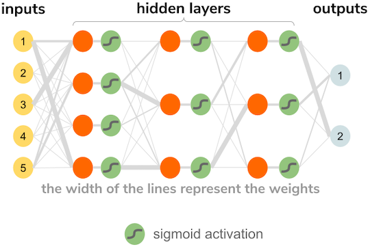
I restricted the model to be sequential, and the layers to be only dense / fully connected, this means that every neuron is connected to every neuron of the following layer. Also, as a restriction, the only activation function I implemented was sigmoid:

With my neural network coded, I tested it with a very basic problem, the famous XOR problem.

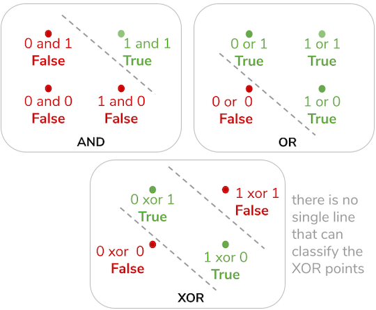
XOR is a logical operation that cannot be solved by a single perceptron because of its linearity restriction:

As you can see, when plotted in an X,Y plane, the logical operators AND and OR have a line that can clearly separate the points that are false from the ones that are true, hence a perceptron can easily learn to classify them; however, for XOR there is no single straight line that can do so, therefore a multilayer perceptron is needed for the task.

For the test I created a neural network with my library:

import Neural_Network as nn

inputs = 3
hidden_layers = [2, 1]
outputs = 1
learning_rate = 0.03

NN = nn.NeuralNetwork(inputs, hidden_layers, outputs, learning_rate)

The three inputs I decided to use (after a lot of trial and error) are the X and Y coordinate of a point (between X = 0, X = 1, Y = 0 and Y = 1) and as the third input the multiplication of both X and Y. Apparently it gives the network more information, and it ends up converging much more quickly with this third input.

Then there is a single hidden layer with 2 neurons and one output value, that will represent False if the value is closer to 0 or True if the value is closer to 1.

Then I created the learning data, which is quite trivial for this problem, since we know very easily how to compute XOR.

training_data = []
for n in range(learning_rounds):
    x = rnd.random()
    y = rnd.random()
    training_data.append([x, y, x * y, 0 if (x < 0.5 and y < 0.5) or (x >= 0.5 and y >= 0.5) else 1])

And off we go into training:

for data in training_data:
    NN.train(data[:3].reshape(inputs), data[3:].reshape(outputs))

The ML library can only train on batches of 1 (another self-imposed coding restriction), therefore only one “observation” at a time, this is why the train function accepts two parameters, one is the inputs packed in an array, and the other one is the outputs, packed as well in an array.

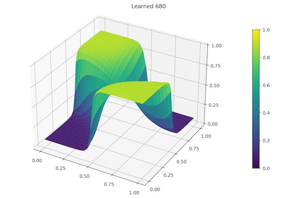
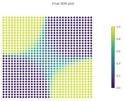
To see the neural net in action I decided to plot the predicted results in both a 3d X,Y,Z surface plot (z being the network’s predicted value), and a scatter plot with the color of the points representing the predicted value.

This was plotted in MatPlotLib, so we needed to do some housekeeping first:

fig = plt.figure()
fig.canvas.set_window_title('Learning XOR Algorithm')
fig.set_size_inches(11, 6)

axs1 = fig.add_subplot(1, 2, 1, projection='3d')
axs2 = fig.add_subplot(1, 2, 2)

Then we need to prepare the data to be plotted by generating X and Y values distributed between 0 and 1, and having the network calculate the Z value:

x = np.linspace(0, 1, num_surface_points)
y = np.linspace(0, 1, num_surface_points)
x, y = np.meshgrid(x, y)

z = np.array(NN.forward_propagation([x, y, x * y])).reshape(num_surface_points, num_surface_points)

As you can see, the z values array is reshaped as a 2d array of shape (x,y), since this is the way Matplotlib interprets it as a surface:

axs1.plot_surface(x, y, z,
                  rstride=1,
                  cstride=1,
                  cmap='viridis',
                  vmin=0,
                  vmax=1,
                  antialiased=True)

The end result looks something like this:

Then we reshape the z array as a one dimensional array to use it to color the scatter plot:

z = z.reshape(num_surface_points ** 2)
scatter = axs2.scatter(x, y,
                       marker='o',
                       s=40,
                       c=z.astype(float),
                       cmap='viridis',
                       vmin=0,
                       vmax=1)

To actually see the progress while learning, I created a Matplotlib animation, and it is quite interesting to see as it learns.

So my baby ML library is completed for now, but still I would like to enhance it in several ways:

• include multiple activation functions (ReLu, linear, Tanh, etc.)
• allow for multiple optimizers (Adam, RMSProp, SGD Momentum, etc.)
• have batch and epoch training schedules functionality
• save and load trained model to file

I will get to it soon…

Ghostwritten

我是一名在北京参与内卷工程的 cloud Natvie 工程师，4年工作经验，虽然毕业于一宗古老的中药学科，但更着迷旅行，音乐，摄影。